Pushforward plots in FlexiChains.jl

Published on: 2026-07-22

The text and code presented here are a slightly adapted version of the example I created for the FlexiChains documentation.

These visualisations are inspired by Michael Betancourt’s MCMC visualisation tools. Michael already made them available in R in Python, so check these out if you are working in either of these languages!

Pushfor…-what distribution?

A pushforward distribution is obtained by mapping a function over a distribution: specifically, if some random variable $\theta$ has distribution $p(\theta)$, then the pushforward of $\theta$ through a function $f$ is the distribution of $Y = f(\theta)$.

In Bayesian inference, we’re often interested in taking posterior draws $\theta \sim p(\theta \mid D)$ (as represented in a chain) and pushing this through some function $f$ to obtain a new distribution. For example, $f$ may be the function which generates posterior predictive draws, in which case the pushforward distribution is the posterior predictive distribution.

Each parameter draw $\theta$ yields a different draw of $f$, so the spread of $f$ inherits posterior uncertainty. The pushforward plots in this section visualise that uncertainty as nested quantile bands, displayed as either a fitted curve (pushforward_continuous), per-group summaries (pushforward_discrete), or predictive histograms (pushforward_hist).

using PalmerPenguins, DataFrames, Chain
using Turing, CairoMakie
using StatsBase: denserank, ZScoreTransform, fit, reconstruct
using FlexiChains
using FlexiChains: FM

Set up data

We’ll concoct an example with the Palmer penguins dataset to show how these plots can be used.

standardise(x) = (x .- mean(x)) ./ std(x)

# Load data and normalise continuous variables
df = @chain DataFrame(PalmerPenguins.load()) begin
	dropmissing(_)
	transform(_, names(_, Real) .=> standardise => (x -> "z_$x"))
	transform(_, :species => denserank => :species_idx)
end

Since the model will consume z-standardised values, we later want to unstandardise these again. A nice way to do so is using StatsBase.ZScoreTransform together with StatsBase.reconstruct for this purpose.

bill_zs = fit(ZScoreTransform, Float64.(df.bill_length_mm))
mass_zs = fit(ZScoreTransform, Float64.(df.body_mass_g))

We also want to keep track of the mapping of species indices to species names for legend and axis ticks later.

using OrderedCollections: OrderedDict
species = sort(OrderedDict(Pair.(unique(df.species_idx), unique(df.species))))

Turing model

We’ll define a model for penguin bill length as a function of species and body mass.

@model function bill_model(species, body_mass)
    n_species = length(unique(species))
    β1 ~ filldist(Normal(0, 1), n_species)
    β2 ~ Normal(0, 1)
    β3 ~ filldist(Normal(0, 1), n_species)
    σ ~ Exponential(1)
    μ = @. β1[species] + β2 * body_mass + β3[species] * body_mass
    bill_length_mm ~ MvNormal(μ, σ)
end

We model a penguin’s bill length as a function of its species (β1), its body mass (β2), and the interaction between them (β3), i.e., we ask “does the effect of body mass vary by species?”.

Next, we condition the model on the observed data and run MCMC.

prior_model = bill_model(df.species_idx, df.z_body_mass_g)
cond_model = prior_model | (; bill_length_mm=df.z_bill_length_mm)
chain = sample(cond_model, NUTS(0.9), MCMCThreads(), 1000, 4)

Posterior predictive distribution

A common starting point is to plot the posterior predictive distribution (see also the Turing.jl docs on this); it can help us (at least superficially) test if the model captured basic patterns in the input data.

We can plot a summary histogram with uncertainty bands using pushforward_hist. By specifying the observed keyword argument we can also overlay the observed data so that we can visually compare the two distributions.

Note that we pass the prior_model here, not the conditioned model, so that we can sample new draws for the conditioned variables (i.e., bill length). This is explained in the Turing docs linked above.

using FlexiChains: transform_values

ppd = @chain prior_model begin
	predict(_, chain)
	transform_values(_, :bill_length_mm => (v -> reconstruct(bill_zs, v)))
end

fig = Figure()
ax = Axis(fig[1, 1])
FM.pushforward_hist!(ppd, @varname(bill_length_mm); observed=df.bill_length_mm)
ax.xlabel = "Bill length (mm)"
ax.title = "Posterior predictive distribution"
fig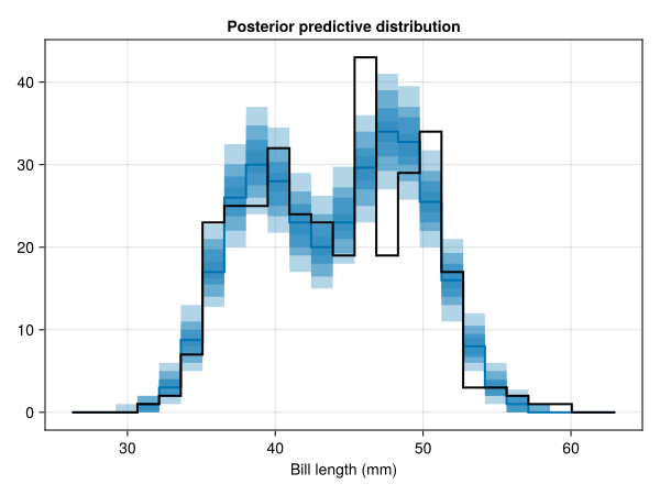

Fitted curves

We may also be interested in how predicted bill length changes with increasing body mass, and how this varies by species. For this, we can make use of pushforward_continuous by feeding it a grid of body mass values.

In the example below, we have set σ = 0 to drop the predictive uncertainty; we’re interested only in the uncertainty of the means here.

We will begin by setting up a grid of body mass values to predict for. We’re intentionally creating an equally spaced grid here to allow us to plot bill length as a function of body mass.

Next, we create an artificial armada of penguins of 50 individuals per species (nah, not really… real colonies are muuuch larger!).

pred_species = repeat(1:3, inner=50)
pred_body_mass = repeat(range(-3.3, 3.3, length=50), outer=3)
pred_model = fix(bill_model(pred_species, pred_body_mass), (; σ=0))

pred = @chain pred_model begin
	predict(_, chain)
	transform_values(_, :bill_length_mm => (v -> reconstruct(bill_zs, v)))
end

colors = first(Makie.wong_colors(), length(species))
fig = Figure()
ax = Axis(fig[1, 1]; xlabel="Body mass (g)", ylabel="Bill length (mm)", 
          limits=(extrema(df.body_mass_g), nothing))

# Iteratively plot predicted bands
for (s, color) in zip(1:3, colors)
    ix = findall(==(s), pred_species)
    x_grid = reconstruct(mass_zs, pred_body_mass[ix])
    FM.pushforward_continuous!(ax, pred, @varname(bill_length_mm[ix]); 
                               x_grid, color)
end

# Plot observed weight-length pairs
for (s, color) in zip(1:3, colors)
    sdf = subset(df, :species_idx => ByRow(==(s)))
    scatter!(sdf.body_mass_g, sdf.bill_length_mm; color=(color, 0.3))
end

# Create legend
elems = [PolyElement(; color=c) for c in colors]
labels = collect(values(species))
axislegend(ax, elems, labels, position=:lt)

fig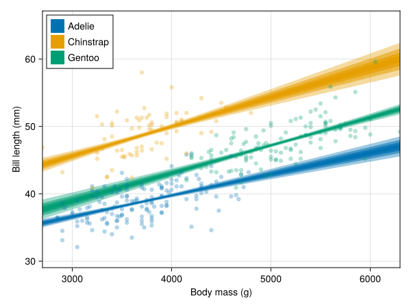

Per-group summary

Finally, if we want to examine the distributions of discrete parameters, such as the main or interaction effect of species, we can use pushforward_discrete. Here, we’ll look at the interaction effect to see if there’s any evidence for the effect of body mass varying by species.

fig = Figure()
ax = Axis(fig[1, 1], limits=(nothing, (-1.1, 1.1)))
FM.pushforward_discrete!(chain, @varname(β3))
ax.xticks = (1:3, "β3[" .* collect(values(species)) .* "]")
fig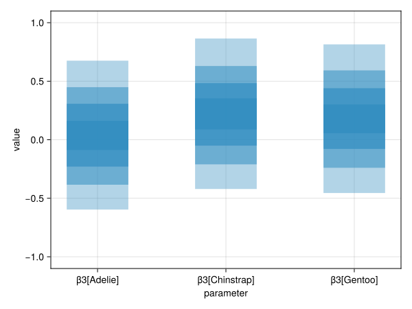

It seems that any between-species variation in the effect of body mass on bill length is at best moderate.